Euler Examples

Search

Double Pendulum

The formulas and their derivation are from

Wikipedia

>function f(x,y) ...
 th1=y[1]; th2=y[2]; dth=th1-th2; c=cos(th1-th2);
 l=1; g=10; m=1; ml2=m*l^2;
 pth1=y[3]; pth2=y[4];
 Dth1=6/ml2*(2*pth1-3*c*pth2)/(16-9*c^2);
 Dth2=6/ml2*(8*pth2-3*c*pth1)/(16-9*c^2);
 return [Dth1,Dth2,
    -ml2/2*(Dth1*Dth2*sin(th1-th2)+3*g/l*sin(th1)),
    -ml2/2*(-Dth1*Dth2*sin(th1-th2)+g/l*sin(th2))]
 endfunction

>t=0:0.01:50;
>s=ode("f",t,[0,0,4,4]); s=s[1:2]-pi/2;

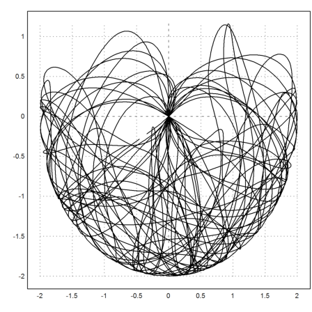
The next plot shows all positions reached from the end of the second axis.

>plot2d(cos(s[1])+cos(s[2]),sin(s[1])+sin(s[2])):

>t=0:0.05:50;
>s=ode("f",t,[0,0,4,4]); s=s[1:2]-pi/2;

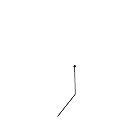
We animate this.

>function anim (th1,th2) ...
 setplot(-2,2,-2,2);
 loop 1 to cols(th1)
    clg;
    a=th1[#]; b=th2[#];
    lw=linewidth(3);
    hold on;
    plot([0,cos(a),(cos(a)+cos(b))],
        [0,sin(a),(sin(a)+sin(b))]);
    markerstyle("o#");
    mark(0,0);
    hold off;
    linewidth(lw);
    wait(0);
    if testkey() then break; endif;
 end;
 endfunction

Press any key to sto the animation.

>anim(s[1],s[2]):

I have uploaded the animation to YouTube.

YouTube Channel for Euler Math Toolbox

Examples